There are many applications that require the measurement of current. Many digital multimeters can measure up to 10 A with a high degree of precision. However, if higher currents need to be measured, other methods must be used. While it is a simple matter to insert a current sensing resistor in series with the load and measure the voltage drop across it, there is a trade-off. The voltage across the sense resistor should be small enough to provide the maximum voltage to the load and to minimize the heat dissipation in the sense resistor, but must be large enough to enable the voltage across the sense resistor to be measured with a high degree of accuracy. There is the added problem of measuring a voltage with, for example, an oscilloscope where the earth lead is not ground referenced. The circuit described in this article facilitates the measurement of a low voltage across the sense resistor and produces an amplified, ground-referenced output voltage with a high level of accuracy.
The Circuit
The circuit shown in Figure 1 uses the LTC6102 and an Isabellenhütte* 50 µΩ current shunt. The current in the load develops a voltage across sense resistor R1. This device has a feedback loop that keeps +IN and –INS at the same voltage by sinking current into the –INF pin. Therefore, the voltage across R1 is the same as the voltage across R2. Thus, the current through R2 is lower than the load current by the ratio of R2 to R1. This current flows through the OUT pin and develops a voltage across R3 that can then be measured.
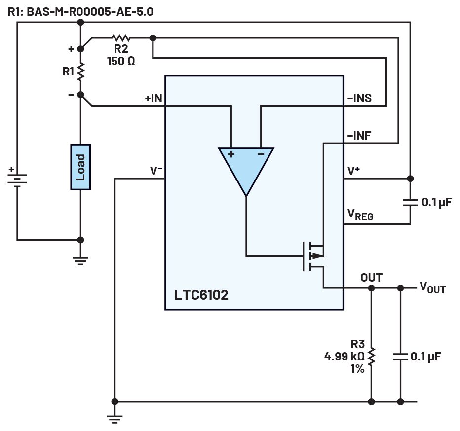
Figure 1. The current sense circuit.
The output voltage is represented by Equation 1.
Likewise, with Equation 2.
*As a point of trivia, Isabellenhütte is supposedly the oldest electronics company in the world.
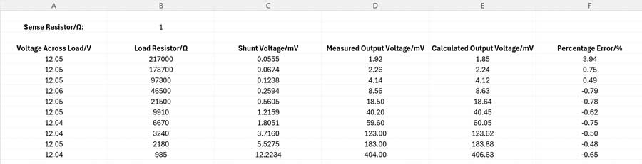
Figure 2. Output voltage and error vs. shunt voltage.
Measuring DC
Rather than evaluate the circuit using a high current, the 50 µΩ shunt can be replaced with a 1 Ω precision resistor, and therefore the circuit generates the same output voltage, but with load resistors that are 20,000× higher. Also, using high value load resistors means the impedance of the test leads does not affect the resistance readings. The voltage across the load resistor and the resistance of the load can both be measured using a standard multimeter, and hence the load current can be calculated to a high degree of precision.
The voltage across the 1 Ω shunt can thus be calculated at various load currents. The output voltage of the part can then be measured using either an oscilloscope or a voltmeter. Figure 2 shows a table of test results taken at various loads using a 1 Ω, 1% resistor as the shunt. The readings in columns A, B, and D are measured using a calibrated multimeter. Column C is calculated by dividing the voltage across the load (column A) by the measured load resistance (column B), then multiplying by the sense resistor. Column E is calculated by dividing the shunt voltage by 150 (R2) and multiplying by 4990 (R3). Column F is calculated by subtracting the calculated output voltage (column E) from the measured output voltage (column D), then dividing by the calculated output voltage.
Figure 3 shows the output voltage plotted against the shunt voltage. The right axis shows the percentage error between the calculated output voltage and the measured output voltage
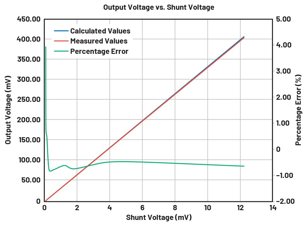
Figure 3. Output voltage and error vs. shunt voltage.
The input offset voltage adds an error to the voltage measured across the sense resistor, so the voltage across the sense resistor must be significantly higher than the offset voltage. As an example, if the voltage across the sense resistor is 100 mV, an input offset voltage in the current sense amplifier of 1 mV would create a 1% error in the readings. However, while a higher voltage across the shunt produces a more accurate result, it also increases the heat dissipation in the shunt and lowers the voltage to the load. A high offset voltage also limits the dynamic range of load currents that can be accurately measured. As the load current decreases, the voltage across the shunt gets smaller, and the input offset voltage adds proportionately more error.
The device’s input offset voltage is 10 µV, so it contributes very little error to the measurement and ensures that a wide dynamic load current can be measured. As can be seen in Figure 2 and Figure 3, the offset voltage starts adding significant error when the sense voltage falls below 55 µV.
Calibration
Figure 2 shows that a load resistor of 985 Ω produces a shunt voltage of 12.2234 mV. The input offset voltage is insignificant compared to the shunt voltage, so it does not contribute to the reading error. The system can now be calibrated. R3 can be adjusted to create a measured voltage equal to the calculated output voltage of 406.63 mV, thus calibrating out the errors in resistors R1, R2, and R3.
Figure 2 shows that the error at high currents is –0.65% and the error at low currents is +3.94%. If the system is calibrated, by adjusting R3, then the error at low currents will be +4.59%, so the measured output voltage should now read 1.935 mV. The difference between the calculated output voltage and the new measured output voltage enables the input offset voltage to be calculated, as seen in Equation 3.

This agrees with the data sheet value for the input offset voltage of approximately 3 µV.
MeasuringAC
The LTC6102 is good for measuring DC to a high level of precision, but what about its ability to measure AC? A buck converter’s input current has a large AC content, and if its efficiency is to be determined, the IC must measure this current with a high degree of precision.
Figure 4 shows the frequency response.
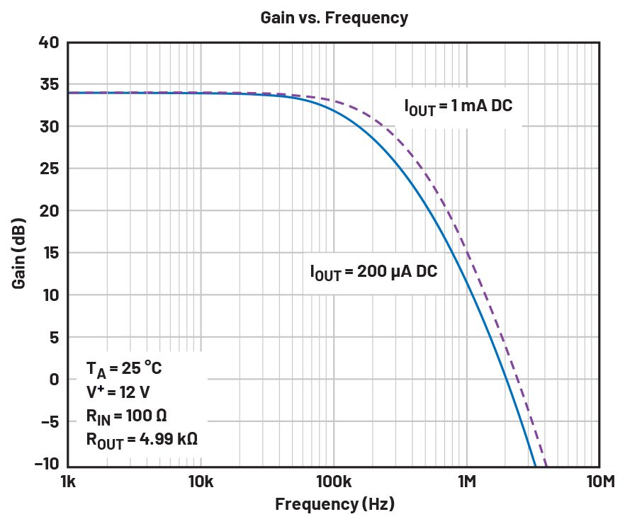
Figure 4. The gain vs. frequency of the LTC6102.
Many DC-to-DC converters switch at a frequency between 200 kHz and 500 kHz, and Figure 4 shows that the attenuation is not significant at these frequencies, so the output of the part will show ripple when measuring the input current of a buck converter. However, this attenuation can be greatly increased by adding a capacitor across output resistor R3, as shown in Figure 1.
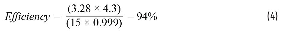
To validate if this is accurate, an LTC3891 buck converter with an input voltage of 15 V and an output voltage of 3.3 V was connected to a load of 4.3 A and the circuit of Figure 1 was inserted in the input line. The 50 µΩ sense resistor was replaced by seven 1 Ω resistors in parallel to give a shunt resistance of 142.8 mΩ. The voltage across the shunt resistors was measured and is shown in Figure 5.
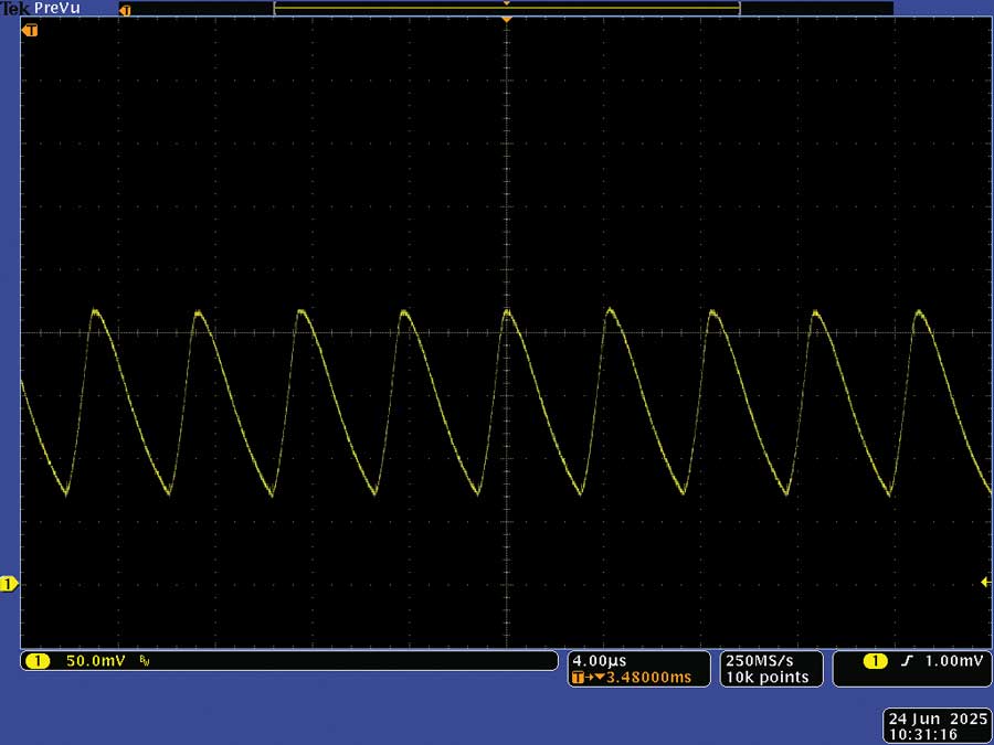
Figure 5. The voltage across the 143mΩ sense resistor.
An RC filter consisting of a 47 Ω resistor and a 10 µF capacitor was placed across the sense resistors and the voltage across the filter capacitor was measured, as shown in Figure 6. This enabled the input current to be measured more accurately with a multimeter, but without changing the value of the shunt resistor.
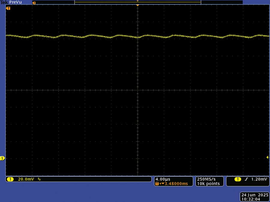
Figure 6. The filtered voltage across the sense resistor.
The voltage across the 10 µF capacitor was measured as 143.6 mV, which corresponds to an input current of 1.005 A.
Then the output voltage of the LTC6102 was measured. Figure 7 shows the output voltage without the 0.1 µF capacitor across R3.

Figure 7. The unfiltered output voltage.
Adding a 0.1 µF capacitor across R3 enabled the output voltage to be measured more accurately, as shown in Figure 8.
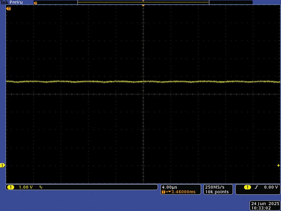
Figure 8. The output voltage with 100nF across R3.
The output voltage across R3 was measured at 4.75 V using a multimeter. This equates to a shunt voltage of 142.79 mV and hence a shunt current of 0.999 A, which is close to the previously measured current of 1.005 A. It is interesting to note that the percentage difference between these two currents is –0.57%, similar to the error shown in the table in Figure 2.
From here, we can work out the efficiency of the LTC3891 with a measured output voltage of 3.28 V, as seen in Equation 4.
Measuring High Currents
The circuit in Figure 1 was used. Thirty 4.7 Ω resistors were wired in parallel to create a 156.6 mΩ load. Copper wire of 10 cm long with a cross-sectional area of 10 mm2 was used to connect them. Copper has a resistivity (ρ) of 1.68 × 10⁻⁸ mΩm and from this, the resistance of the copper wire can be calculated, as seen in Equation 5.
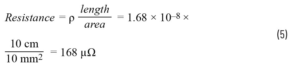
Therefore, the copper wire added negligible resistance to the load.
Figure 9 shows the shunt circuit connected to a car battery. A hot air gun was used to solder the wires to the shunt.
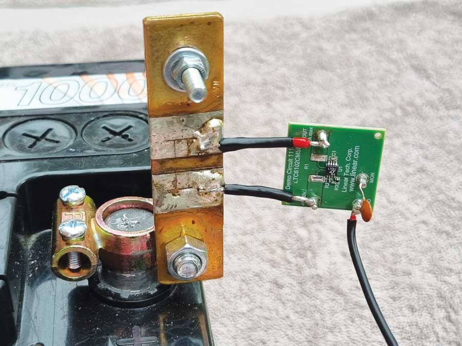
Figure 9. The complete current sense circuit.
Voltmeters were connected across the load and the output of the LTC6102 as shown in Figure 10. An output voltage of 115.4 mV corresponds to a load current of 69.38 A. The calculated load current for a 10.76 V battery is 68.68 A, so the device is measuring the current to an accuracy of 1%.
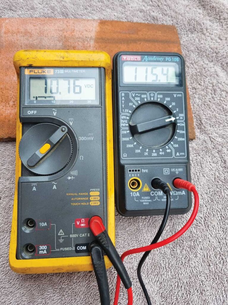
Figure 10. The battery voltage and output from the LTC6102.
On a note about precision, R2 in Figure 1 has a tolerance of 5% as does the 50 µΩ shunt. If the system were to be calibrated at high currents, then the resistance of each load resistor should be measured, so the effective parallel resistance can be calculated. Once the load resistance is known to a high degree of precision, the load voltage can be measured and hence the true accuracy of the system can be determined when operating at high currents.
Conclusion
As can be seen from the figures, the LTC6102 presents a small form factor solution for measuring very high currents and producing a ground-referenced output. The 50 µΩ shunt used in Figure 1 can dissipate up to 36 W, meaning this circuit can be used to measure load currents up to 800 A with a high degree of precision. The device is rated at 60 V (the LTC6102HV is rated at 105 V), providing an excellent solution for a wide variety of applications.
About the Author
The article has been written by Simon Bramble, Principal Applications Engineer at Analog Devices. He graduated from Brunel University in London in 1991 with a degree in electrical engineering and electronics, specializing in analog electronics and power. He has spent his career in analog electronics and worked at Maxim and Linear Technology (both now part of Analog Devices).